
Open the spreadsheet with the data you want to graph. Open Excel (it’s in the All Apps area of the Start menu in Windows and the Applications folder in macOS), then click the file you want to edit.
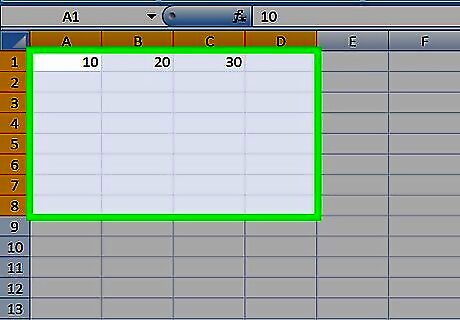
Select the data you want to include in the graph. To do this, click and drag the mouse across all of the data, including the column headers.
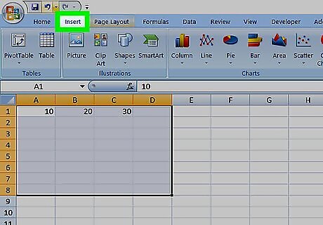
Click the Insert menu. It’s near the top-left corner of the ribbon bar at the top of Excel.
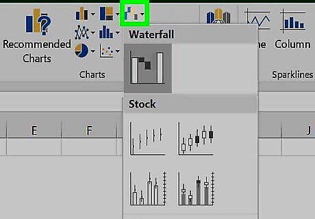
Click the Waterfall Chart icon. It’s in the “Charts” group in the ribbon bar. It’s the 3rd icon after “Recommended Charts” in the top row, and looks like 4 vertical bars of varying heights in a waterfall pattern.
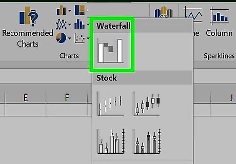
Click the Waterfall Chart icon under the “Waterfall” header. It’s the first icon on the menu. Your data now appears in a waterfall chart on the spreadsheet.
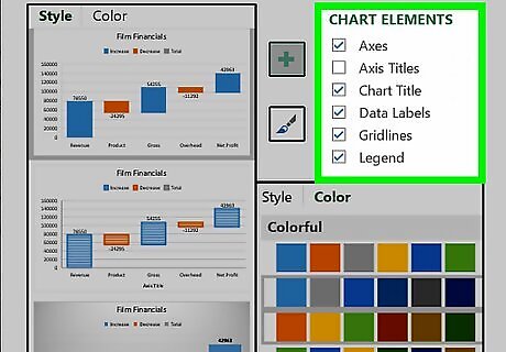
Drag the chart to the desired location. You can now customize the chart to your liking. To customize the chart, click it once to select it, then click DESIGN and/or FORMAT under the “Chart Tools” header in the ribbon bar.


Comments
0 comment