3 Simple Ways to Name a Column in Microsoft Excel

Adding Column Headers

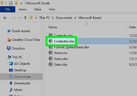
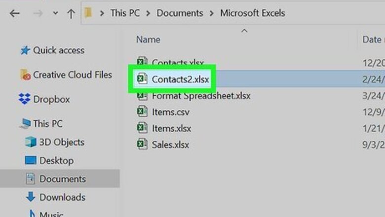
Open a workbook in Microsoft Excel. You can use an existing project or create a new spreadsheet. Make sure you're on the correct worksheet. Microsoft Excel is available on Windows and Mac. You can also use the online web version at https://www.office.com/.

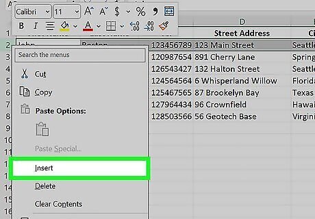
Insert a new row for the names. If you want it at the very top of the page, click 1 on the left side of the spreadsheet to highlight the entire first row. Right-click the first cell, and click Insert. This will place a blank row above your data. If you want the new row in another location, select the row number of the location. Right-click the first cell, and click Insert. If you already have a row for the names, skip to the next step.

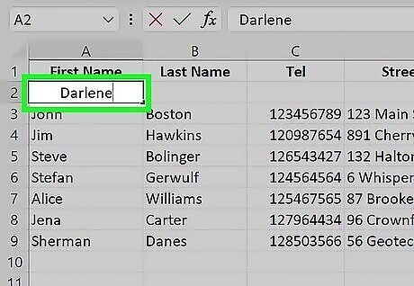
Double-click the first cell and enter a name. This will be the title of the first column.

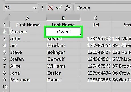
Double-click the next cell and enter a name. You can also press Tab to skip to the next cell in the column. Repeat this for any remaining title cells. If you only have one column to name, skip this step. The headers at the top (letters A-Z) will not change since these are Excel’s way of keeping track of information within your document. However, when you type in a name for column A1, that will become the name for the rest of the “A” column. If you want to see the titles as you scroll down, do the following: Click View at the top. Click Freeze Panes. Click Freeze Top Row.

Changing Column Names to Numbers

Open Microsoft Excel. You can use an existing project or create a new spreadsheet. Use this method if you want to turn the column names (letters A-Z) into numbers instead.

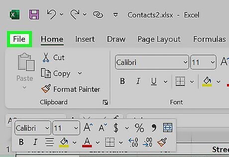
Select File and click Options. This will be at the bottom of the left panel. On Mac, you'll need to click Excel and then Preferences.

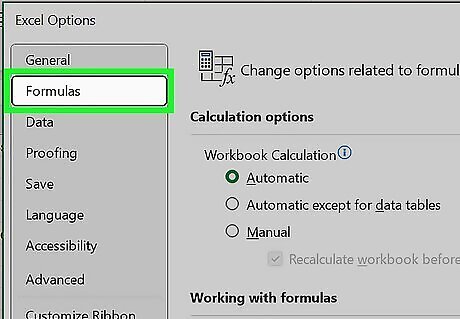
Click Formulas. This is in the left panel. On Mac, click General.

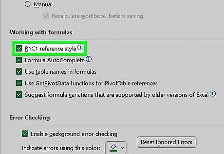
Check the box for "R1C1 reference style". This is underneath the Working with formulas header.

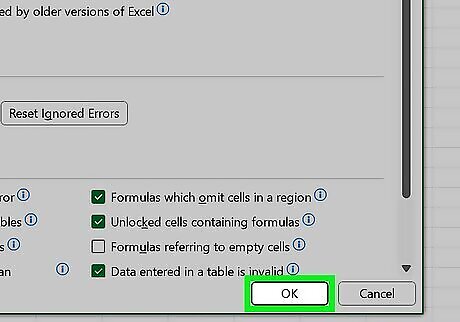
Click OK. This is at the bottom-right corner of the window. The header columns will change from letters to numbers.

Using Power Query

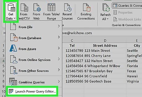
Open the Power Query Editor. Power Query is an add-on you can use in Excel. This allows you to import data through other sources.

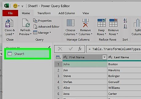
Open a query. You can do this by using a previously loaded query in the Editor, or you can click a cell in the data, select Query, then click Edit.

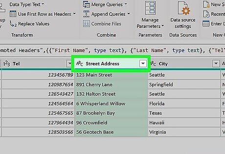
Select the column you want to name. It will be highlighted.

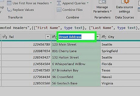
Double-click the column header. This will allow you to rename it. You can also select Transform, then Rename at the top.

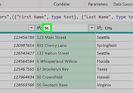
Enter the new column name. This will name the header. Keep in mind that renaming a column header won't rename the original data source header. If the original data source header changes, it can cause query errors.