4 Easy Ways to Keep Leading and Trailing Zeros in Excel

Using Get & Transform

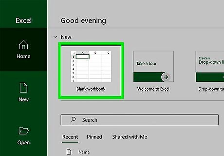
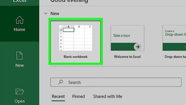
Open a new, blank workbook. The Get & Transform tool (also called Power Query) allows you to customize the data you import from a data source. This tutorial will cover importing from a text file, but the steps will work for other source types as well! Excel automatically and permanently removes leading zeros when you import data into a workbook. The Get & Transform utility allows you to designate certain columns as text during the data importing process. This keeps the leading zeros intact. Alternatively, you can open an existing workbook if you have one that you want the data to be imported to. Refer to our article on downloading Excel if you need to get Excel on a new device.

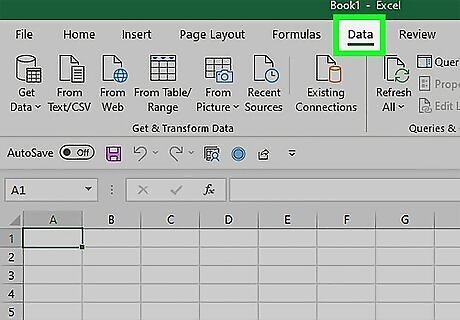
Go to the Data tab.

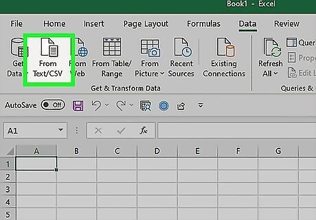
Click From Text/CSV. This option is located next to the Get Data button. If you don’t see this option, you may have a version of excel that is arranged differently. Follow the method below (Importing Data as Text) instead.

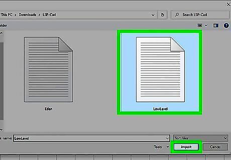
Browse to and select your text file. Then press Import. This will open a preview menu for the data you’re importing into your workbook.

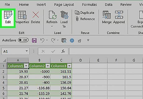
Click Edit. This will start the Query Editor.

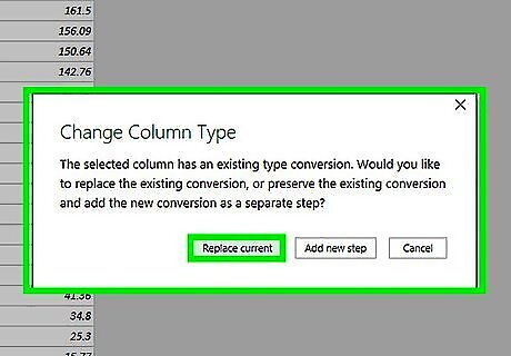
Click the column header for the variable you want to keep as text. Then follow these steps to convert the column to text: Go to the Home tab. Locate the Transform section. Click Data Type. Choose Text. This will open a confirmation “Change Column Type” window. Click Replace Current in the Change Column Type window. Repeat this process for any columns with leading zeros that you want to keep. You can do this for several columns at the same time by selecting multiple column headers with Ctrl + Left-Click.

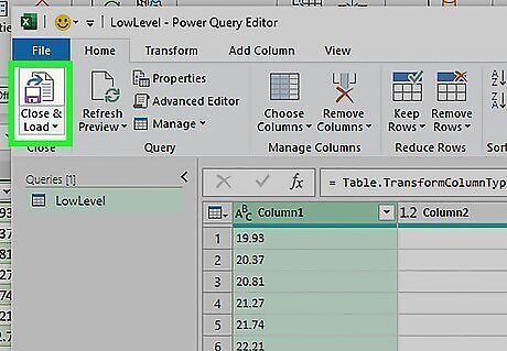
Click Close & Load. Excel will import the data into your worksheet. Check your columns to make sure the leading zeros you want to keep are present. Now you’re ready to make some tables or concatenate some text!

Importing a Data Text File

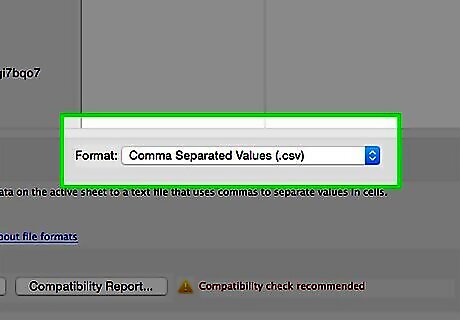
Save a large database in text format. Once you import data into a default Excel workbook, the leading and trailing zeros disappear permanently. The easiest way to fix this is to clear the faulty data and start again. Return to your original database and save it as a .csv file or a .txt file.

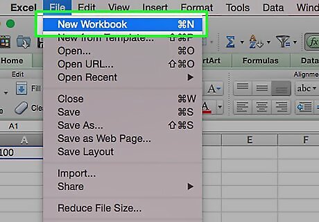
Create a new Excel workbook. You will import your data into this workbook as text, meaning it will not be usable in formulas. You will, however, keep the formatting. This method does allow you to import some columns as text and some columns as numbers. Only the text columns will keep leading and trailing zeros.

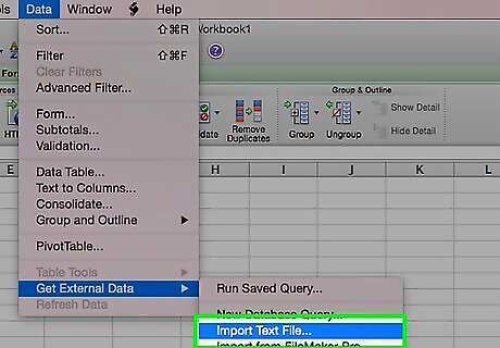
Open the Text Import Wizard. Click the Data tab on your ribbon menu, then look in the External Data Sources section. Click the icon labeled Text or From Text.

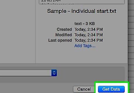
Import data from the text document. Select the text file in the "Choose a File" window. Follow the onscreen instructions to complete Steps 1 and 2.

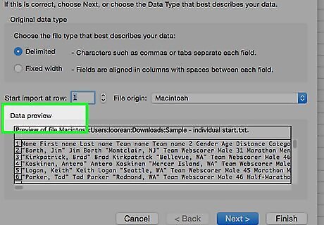
Set columns to text format. In Step 3 of the Text Import Wizard, you should see a preview of your spreadsheet. Click on a column to select it, then select an option to set the format for that column. Specifically, to keep leading and trailing zeros in columns containing phone numbers and similar data, select those columns and choose Text. You can now complete the import and load your spreadsheet with the zeros, as intended.

Creating Custom Formats

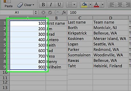
Select the cells you need to change. A custom number format specifies the exact format for your data, including the number of leading or trailing zeroes. To begin, select the columns, rows, or groups of cells you'd like to change.

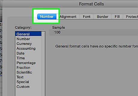
Open the Format window. Click the Home tab on the ribbon and look in the Number group. On Excel for Windows, click the dialog launcher next to the word Number (a small arrow in a square). On Excel for Mac, click the dropdown menu (it says General by default) and select Custom.... On old versions of Excel without a ribbon menu, instead click Format → Cells → Number tab.

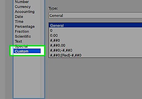
Create a custom format. In Excel 2013 and Excel 2016, just select any format on the list. When you edit that default format, Excel will automatically create a new custom format without altering the default option. On all other versions of Excel, select Custom from the list of options instead. Look for a text box labeled Type where you can enter your custom format. If your data represents calendar dates, phone numbers, or other common data types, browse the list of default options. You may be able to use one of them rather than creating your own format.

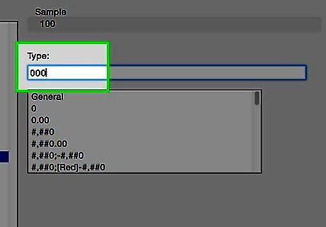
Add leading zeroes. Custom formats use several "placeholder characters" to specify how digits should display. The character 0 (zero) tells Excel to display a zero in that position if there is no other digit there. For example, the format 000 will add leading zeroes to the hundreds and tens place if necessary. 97 will display as 097, and 3 will display as 003. Numbers to the left of the decimal point are always displayed. Even though there are only three digits in the format code 000, the number 3750 will still display as 3750.

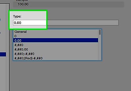
Specify decimal places and trailing zeroes. Custom number formats will delete all digits after the decimal point unless you specify otherwise. To change this, just add a decimal point to the end of your custom code, followed by 0 (or one of the placeholder characters described below). For example, 000.000 will round to the nearest thousandth, and add up to three trailing zeros after the decimal point. Here's how various numbers look in the 000.000 format: 13.1 becomes 013.100 95001 becomes 95001.000 5.0057 becomes 5.006

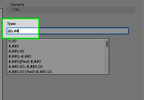
Use the pound sign to prevent extra zeroes. The symbol # is another placeholder character in custom formats. This will prevent all leading zeroes if used at the front of the number, and prevent all trailing zeroes if used after the decimal point. For example, the custom format 00.## allows for a leading zero in the tens place, but no trailing zeroes: 5.8 becomes 05.8 2.71 becomes 02.71 15.0 becomes 15 38.315 becomes 38.32

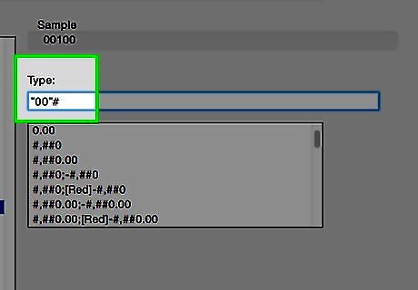
Add leading zeros as text. Excel treats anything inside quotation marks as text in your custom format, and will display it exactly as you typed it. This may be useful if each cell in your original database had exactly two leading zeros, for example. To restore these, set your spreadsheet to the custom format "00"#. If your data includes digits after a decimal point, prevent rounding by using the custom format "00"#.## instead, using as many # or 0 characters after the decimal point as necessary.

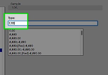
Align decimal points with a question mark. If your goal is to align the decimal points in a column, there's no need to add leading or trailing zeroes. Use the ? character in your custom format, and Excel will add empty spaces instead to align the digits in the column. For example: ?.??? rounds to the nearest thousandth with no trailing zeroes, and aligns the decimal points. 000.? adds leading zeros up to the thousands place, rounds to the nearest tenth with no trailing zeros, and aligns the decimal points. ?.00 rounds to the nearest hundredth with trailing zeros and aligns the decimal points.