How to Calculate Averages in Excel

Netell

Editor

posted on 10 years ago — updated on 1 second ago

26
views

Mathematically speaking, “average” is used by most people to mean “central tendency,” which refers to the centermost of a range of numbers. There are three common measures of central tendency: the (arithmetic) mean, the median, and the mode. Microsoft Excel has functions for all three measures, as well as the ability to determine a weighted average, which is useful for finding an average price when dealing with different quantities of items with different prices.

Steps

Finding the Arithmetic Mean (Average) Value

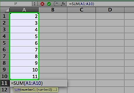
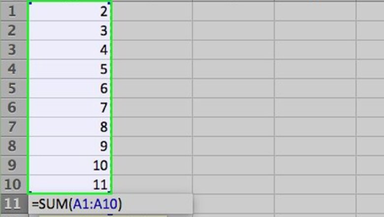
Enter the numbers you want to find the average of. To illustrate how each of the central tendency functions works, we’ll use a series of ten small numbers. (You won’t likely use actual numbers this small when you use the functions outside these examples.) Most of the time, you’ll enter numbers in columns, so for these examples, enter the numbers in cells A1 through A10 of the worksheet. The numbers to enter are 2, 3, 5, 5, 7, 7, 7, 9, 16, and 19. Although it isn’t necessary to do this, you can find the sum of the numbers by entering the formula “=SUM(A1:A10)” in cell A11. (Don’t include the quotation marks; they’re there to set off the formula from the rest of the text.)

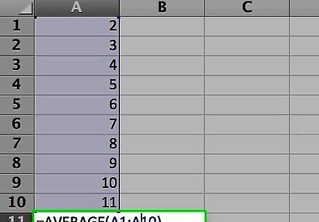
Find the average of the numbers you entered. You do this by using the AVERAGE function. You can place the function in one of three ways: Click on an empty cell, such as A12, then type “=AVERAGE(A1:10)” (again, without the quotation marks) directly in the cell. Click on an empty cell, then click on the “fx” symbol in the function bar above the worksheet. Select “AVERAGE” from the “Select a function:” list in the Insert Function dialog and click OK. Enter the range “A1:A10” in the Number 1 field of the Function Arguments dialog and click OK. Enter an equals sign (=) in the function bar to the right of the function symbol. Select the AVERAGE function from the Name box dropdown list to the left of the function symbol. Enter the range “A1:A10” in the Number 1 field of the Function Arguments dialog and click OK.

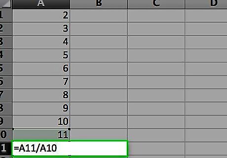
Observe the result in the cell you entered the formula in. The average, or arithmetic mean, is determined by finding the sum of the numbers in the cell range (80) and then dividing the sum by how many numbers make up the range (10), or 80 / 10 = 8. If you calculated the sum as suggested, you can verify this by entering “=A11/10” in any empty cell. The mean value is considered a good indicator of central tendency when the individual values in the sample range are fairly close together. It is not considered as good of an indicator in samples where there are a few values that differ widely from most of the other values.

Finding the Median Value

Enter the numbers you want to find the median for. We’ll use the same range of ten numbers (2, 3, 5, 5, 7, 7, 7, 9, 16, and 19) as we used in the method for finding the mean value. Enter them in the cells from A1 to A10, if you haven’t already done so.

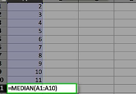
Find the median value of the numbers you entered. You do this by using the MEDIAN function. As with the AVERAGE function, you can enter it one of three ways: Click on an empty cell, such as A13, then type “=MEDIAN(A1:10)” (again, without the quotation marks) directly in the cell. Click on an empty cell, then click on the “fx” symbol in the function bar above the worksheet. Select “MEDIAN” from the “Select a function:” list in the Insert Function dialog and click OK. Enter the range “A1:A10” in the Number 1 field of the Function Arguments dialog and click OK. Enter an equals sign (=) in the function bar to the right of the function symbol. Select the MEDIAN function from the Name box dropdown list to the left of the function symbol. Enter the range “A1:A10” in the Number 1 field of the Function Arguments dialog and click OK.

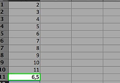
Observe the result in the cell you entered the function in. The median is the point where half the numbers in the sample have values higher than the median value and the other half have values lower than the median value. (In the case of our sample range, the median value is 7.) The median may be the same as one of the values in the sample range, or it may not.

Finding the Mode Value

Enter the numbers you want to find the mode for. We’ll use the same range of numbers (2, 3, 5, 5, 7, 7, 7, 9, 16, and 19) again, entered in cells from A1 through A10.

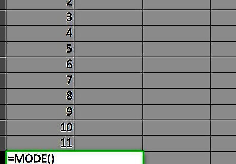
Find the mode value for the numbers you entered. Excel has different mode functions available, depending on which version of Excel you have. For Excel 2007 and earlier, there is a single MODE function. This function will find a single mode in a sample range of numbers. For Excel 2010 and later, you can use either the MODE function, which works the same as in earlier versions of Excel, or the MODE.SNGL function, which uses a supposedly more accurate algorithm to find the mode. (Another mode function, MODE.MULT returns multiple values if it finds multiple modes in a sample, but it is intended for use with arrays of numbers instead of a single list of values.)

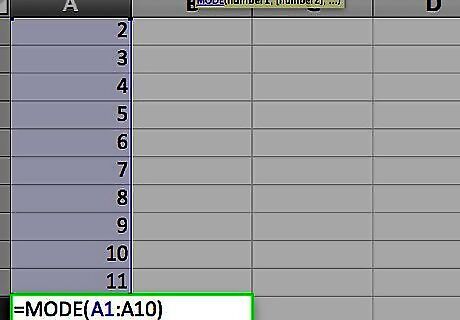
Enter the mode function you’ve chosen. As with the AVERAGE and MEDIAN functions, there are three ways to do this: Click on an empty cell, such as A14 then type “=MODE(A1:10)” (again, without the quotation marks) directly in the cell. (If you wish to use the MODE.SNGL function, type “MODE.SNGL” in place of “MODE” in the equation.) Click on an empty cell, then click on the “fx” symbol in the function bar above the worksheet. Select “MODE” or “MODE.SNGL,” from the “Select a function:” list in the Insert Function dialog and click OK. Enter the range “A1:A10” in the Number 1 field of the Function Arguments dialog and click OK. Enter an equals sign (=) in the function bar to the right of the function symbol. Select the MODE or MODE.SNGL function from the Name box dropdown list to the left of the function symbol. Enter the range “A1:A10” in the Number 1 field of the Function Arguments dialog and click OK.

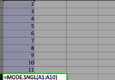
Observe the result in the cell you entered the function in. The mode is the value that occurs most often in the sample range. In the case of our sample range, the mode is 7, as 7 occurs three times in the list. If two numbers appear in the list the same number of times, the MODE or MODE.SNGL function will report the value that it encounters first. If you change the “3” in the sample list to a “5,” the mode will change from 7 to 5, because the 5 is encountered first. If, however, you change the list to have three 7s before three 5s, the mode will again be 7.

Finding a Weighted Average

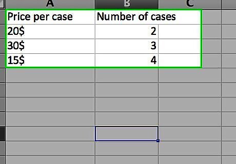
Enter the data you want to calculate a weighted average for. Unlike finding a single average, where we used a one-column list of numbers, to find a weighted average we need two sets of numbers. For the purpose of this example, we’ll assume the items are shipments of tonic, dealing with a number of cases and the price per case. For this example, we’ll include column labels. Enter the label “Price Per Case” in cell A1 and “Number of Cases” in cell B1. The first shipment was for 10 cases at $20 per case. Enter “$20” in cell A2 and “10” in cell B2. Demand for tonic increased, so the second shipment was for 40 cases. However, due to demand, the price of tonic went up to $30 per case. Enter “$30” in cell A3 and “40” in cell B3. Because the price went up, demand for tonic went down, so the third shipment was for only 20 cases. With the lower demand, the price per case went down to $25. Enter “$25” in cell A4 and “20” in cell B4.

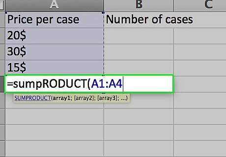
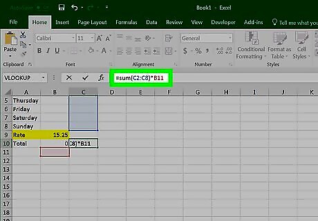
Enter the formula you need to calculate the weighted average. Unlike figuring a single average, Excel doesn’t have a single function to figure a weighted average. Instead you’ll use two functions: SUMPRODUCT. The SUMPRODUCT function multiplies the numbers in each row together and adds them to the product of the numbers in each of the other rows. You specify the range of each column; since the values are in cells A2 to A4 and B2 to B4, you’d write this as “=SUMPRODUCT(A2:A4,B2:B4)”. The result is the total dollar value of all three shipments. SUM. The SUM function adds the numbers in a single row or column. Because we want to find an average for the price of a case of tonic, we’ll sum up the number of cases that were sold in all three shipments. If you wrote this part of the formula separately, it would read “=SUM(B2:B4)”.

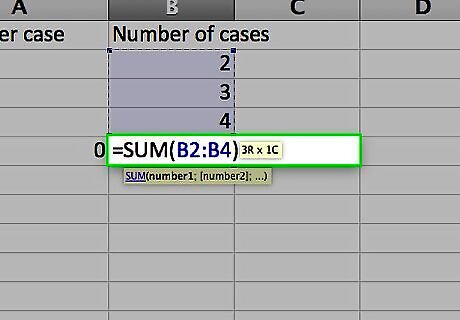
Since an average is determined by dividing a sum of all numbers by the number of numbers, we can combine the two functions into a single formula, written as “=SUMPRODUCT(A2:A4,B2:B4)/ SUM(B2:B4)”.

Observe the result in the cell you entered the formula in. The average per-case price is the total value of the shipment divided by the total number of cases that were sold. The total value of the shipments is 20 x 10 + 30 x 40 + 25 x 20, or 200 + 1200 + 500, or $1900. The total number of cases sold is 10 + 40 + 20, or 70. The average per case price is 1900 / 70 = $27.14.