views
Creating an Amortization Schedule Manually
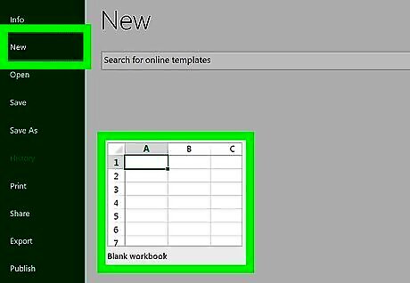
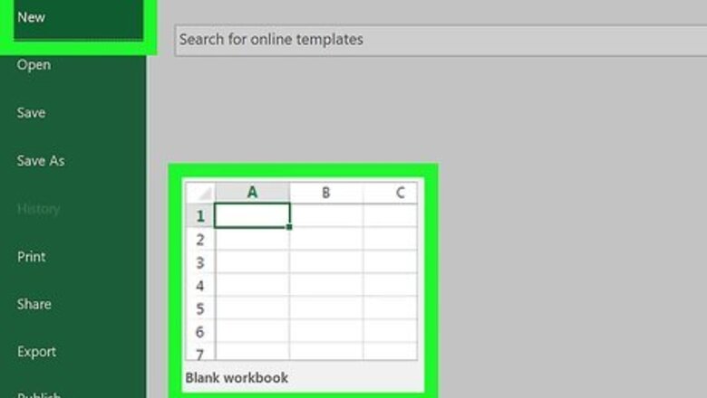
Open a new spreadsheet in Microsoft Excel.
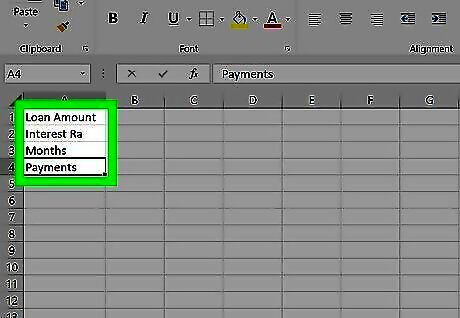
Create labels in column A. Create labels for your data in the first column to keep things organized. Here's what you should put in each cell: . A1: Loan Amount A2: Interest Rate A3: Months A4: Payments
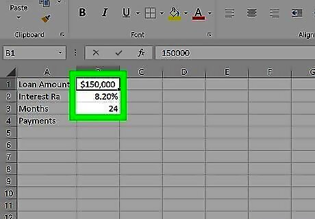
Enter the information pertaining to your loan in column B. Fill out cells B1-B3 with information about your loan. Leave B4 (the cell next to the Payments label) blank. The "Months" value should be the total number of months in the loan term. For example, if you have a 2-year loan, enter 24. The "Interest Rate" value should be a percentage (e.g., 8.2%).
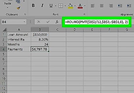
Calculate your payment in cell B4. To do this, click cell B4, and then type the following formula into the formula (fx) bar at the top of the sheet and then press ↵ Enter or ⏎ Return: =ROUND(PMT($B$2/12,$B$3,-$B$1,0), 2). The dollar signs in the formula are absolute references to make sure the formula will always look to those specific cells, even if it is copied elsewhere into the worksheet. The loan interest rate must be divided by 12, since it is an annual rate that is calculated monthly. For example, if your loan is for $150,000 at 6 percent interest for 30 years (360 months), your loan payment will calculate out to $899.33.
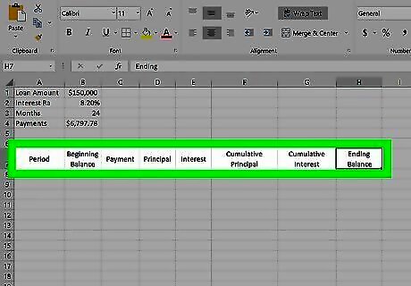
Create column headers in row 7. You'll be adding some additional data to the sheet, which requires a second chart area. Enter the following labels into the cells: A7: Period B7: Beginning Balance C7: Payment D7: Principal E7: Interest F7: Cumulative Principal G7: Cumulative Interest H7: Ending Balance.
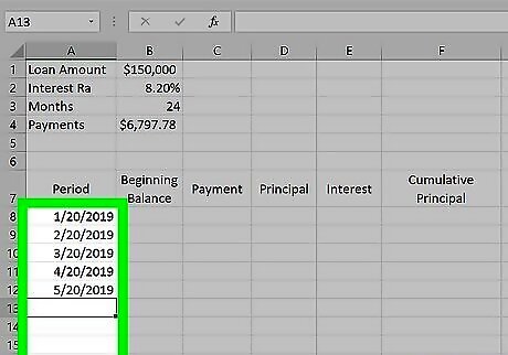
Populate the Period column. This column will contain your payment dates. Here's what to do: Type the month and year of the first loan payment in cell A8. You may need to format the column to show the month and year correctly. Click the cell once to select it. Drag down from the center of the selected cell downward to cover all cells through A367. If this doesn't make all of the cells reflect the correct monthly payment dates, click the small icon with a lightning bolt on it at the bottom-right corner of the bottommost cell and make sure the Last Month option is selected.
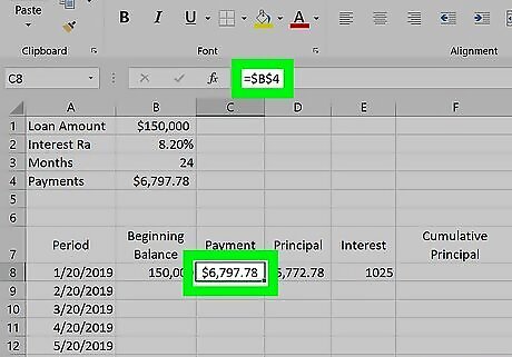
Fill out the other entries in cells B8 through H8. The beginning balance of your loan into cell B8. In cell C8, type =$B$4 and press Enter or Return. In cell E8, create a formula to calculate the loan interest amount on the beginning balance for that period. The formula will look like =ROUND($B8*($B$2/12), 2). The single dollar sign creates a relative reference. The formula will look for the appropriate cell in the B column. In cell D8, subtract the loan interest amount in cell E8 from the total payment in C8. Use relative references so this cell will copy correctly. The formula will look like =$C8-$E8. In cell H8, create a formula to subtract the principal portion of the payment from the beginning balance for that period. The formula will look like =$B8-$D8.
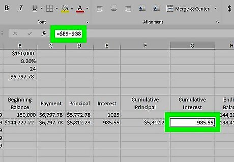
Continue the schedule by creating the entries in B9 through H9. Cell B9 should include a relative reference to the ending balance of the prior period. Type =$H8 into B9 and press Enter or Return. Copy cells C8, D8 and E8 and paste them into C9, D9 and E9 (respectively) Copy H8 and paste it into H9. This is where the relative reference becomes helpful. In cell F9, create a formula to tabulate cumulative principal paid. The formula will look like this: =$D9+$F8. Enter the cumulative interest formula into G9 like this: =$E9+$G8.
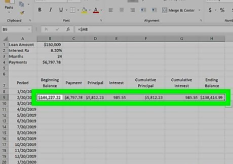
Highlight cells B9 through H9. When you rest the mouse cursor over the bottom-right part of the highlighted area, the cursor will turn to a crosshair.
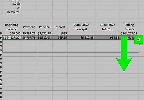
Drag the crosshair all the way down to row 367. This populates all the cells through row 367 with the amortization schedule. If this looks funny, click the small spreadsheet-looking icon at the bottom-right corner of the final cell and select Copy Cells.
Using an Excel Template
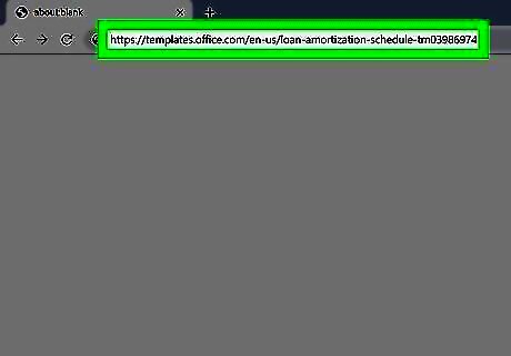
Go to https://templates.office.com/en-us/loan-amortization-schedule-tm03986974. This is a free, downloadable amortization schedule template that makes it easy to calculate the total interest and total payments. It even includes the option to add extra payments.
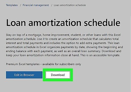
Click Download. This saves the template to your computer in the Excel template format (XLTX).
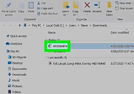
Double-click the downloaded file. It's called tf03986974.xltx, and you'll usually find it in your Downloads folder. This opens the template in Microsoft Excel. The data in the template is there as an example—you'll be able to add your own data. If prompted, click Enable Editing so you can make changes to the workbook.
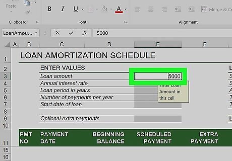
Type the loan amount into the "Loan Amount" cell. It's in the "ENTER VALUES" section near the top-left corner of the sheet. To type it, just click the existing value ($5000) and type your own amount. When you press ⏎ Return or ↵ Enter (or click another cell), the amounts in the rest of the sheet will recalculate. This will happen each time you change a value in this section.
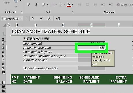
Enter your annual interest rate. This goes into the "Annual interest rate" cell.
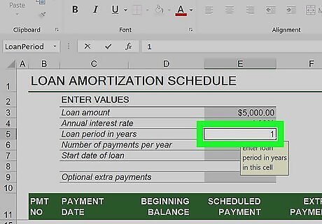
Enter the duration of your loan (in years). This goes into the "Loan period in years" cell.
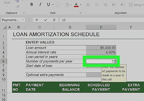
Enter the number of payments you make per year. For example, if you make payments once per month, type 12 into the "Number of payments per year" cell.
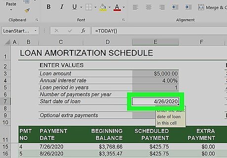
Enter the loan start date. This goes into the "Start date of loan" cell.
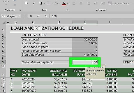
Enter a value for "Optional extra payments." If you pay over the minimum amount due on your loan each pay period, enter that extra amount into this cell. If not, change the default value to 0 (zero).
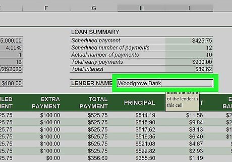
Enter the name of the loan issuer. The default value of the "LENDER NAME" blank is "Woodgrove Bank." Change this to your bank's name for your own reference.
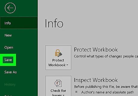
Save the worksheet as a new Excel file. Here's how: Click the File menu at the top-left and select Save As. Select a location on your computer or in the cloud where you'd like to store your schedule. Enter a name for the file. If the file type is not already set to "Excel Workbook (*.xlsx)," select that option from the drop-down menu (below the file name) now. Click Save.


Comments
0 comment